Theory¶

The non-linear shallow water equations (SWE)¶

The tsunami simulation code TsunAWI is based on the rotating non-linear SWE given by the vertically averaged equations of motion and continuity. We consider the boundary value problem in Cartesian coordinates $(x,y)\in\Omega$ in the plane domain $\Omega$ with boundary $\partial\Omega$ at the time $t\in[0,T]$

(1)¶ $\frac{\partial \vec{v}}{\partial t} + f\,\vec{k}\!\times\!\vec{v} + \left(\vec{v}\!\cdot\!\nabla \right) \vec{v} + g\nabla\zeta +\frac r H \,\vec{v} | \vec{v} | - \nabla \left(K_{\!\mathrm{h}} \nabla\vec{v} \right) &= 0,$

(2)¶ $\qquad\qquad\quad \quad\frac{\partial\zeta}{\partial t} + \nabla\cdot \left(H\vec{v}\right) &= 0$

for the horizontal velocity vector $\vec{v} = (u,v)$ and the total water depth $H = h+\zeta>0$ as the sum of the unperturbed water depth $h$ and the surface elevation $\zeta$ . Furthermore, $\nabla = \left( \frac\partial{\partial x}, \frac\partial{\partial y} \right)$ denotes the gradient operator, $f$ the Coriolis parameter, $\vec{k}$ the vertical unit vector, $r$ the bottom friction coefficient, and $K_{\!\mathrm{h}}$ the eddy viscosity coefficient.

Boundary conditions¶

On the solid part of the boundary $\partial\Omega_1$ , the condition

(3)¶ $v_\mathrm{n}\big|_{\partial\Omega_1} &= 0$

for the velocity $v_\mathrm{n}=\vec{v}\times \vec{n}$ normal to $\partial\Omega_1$ is imposed. For the open part $\partial\Omega_2$ , the radiation boundary condition

(4)¶ $v_\mathrm{n}\big|_{\partial\Omega_2} &= \sqrt{\frac g H}\;\zeta$

is implemented in TsunAWI providing free linear wave passage through the open boundary, given the Coriolis acceleration plays only a small role (for a review of several open boundary conditions see [RoedC86]).

Furthermore, as TsunAWI operates on unstructured grids, consider to avoid open boundaries by building a coarse global grid with a finely resolved focus on the region of interest.

For the benchmark problem “Monai Beach channel experiment”, an inflow condition is coded in benchmark.F90.

Numerical implementation¶

Finite element discretization¶

The spatial discretisation of TsunAWI is based on the finite element approach by Hanert et al. [HLRLD05] with modifications like added viscous and bottom friction terms, corrected momentum advection terms, radiation boundary condition, and nodal lumping of mass matrix in the continuity equation.

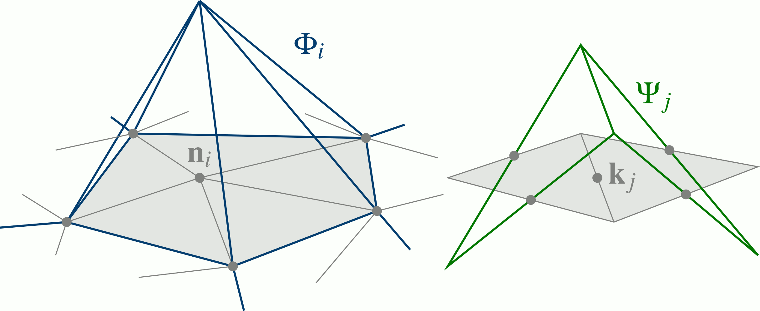
Linear conforming ( $P_1$ ) basis function $\Phi_i$ and linear non-conforming ( $P^\mathrm{NC}_1$ ) basis function $\Psi_j$ for a triangular grid.

The approximated sea surface height $\zeta_h$ and velocity component $u_h$ as linear combinations of the basis functions $\Phi_i$ and $\Psi_j$ , respectively.

The basic principles of discretisation follow [HLRLD05] with linear conforming elements $P_1$ for sea surface height $\zeta$ and water depth $h$ , and linear non-conforming elements $P^\mathrm{NC}_1$ for the velocity $\vec{v}$ . Thus, values for sea surface are computed at element nodes, while the velocity components are regarded at the edges.

Leap-frog time stepping scheme¶

The leap-frog discretisation was chosen as a simple and easily implemented method. We rewrite equations (1) and (2) in time discrete form

$\begin{aligned} \frac{\vec{v}^{\,n+1}-\vec{v}^{\,n-1}}{2{\scriptstyle\triangle}t} + f\, \vec{k}\!\times\! \vec{v}^{\,n} + \left(\vec{v}^{\,n}\!\cdot\! \nabla \right) \vec{v}^{\,n}+ g \nabla \zeta^{\,n} +\frac{r}{H^n}|\vec{v}^{\,n}|\vec{v}^{\,n+1} - \nabla \left(K_{\!\mathrm{h}}\nabla \vec{v}^{\,n-1}\right) & =0\, , \\[.5ex] \frac{\zeta^{n+1} - \zeta^{n-1}}{2 {\scriptstyle\triangle}t} + \nabla \cdot \left(H^n \vec{v}^{\,n} \right)& =0\end{aligned}$

with the time step length ${\scriptstyle\triangle}t$ and the time index $n$ . The leap-frog scheme provides second-order accuracy and is neutral within the stability range. Notice that friction and viscosity contributions deviate from the usual leap-frog method.

This scheme, however, has a numerical mode, which is removed by the standard Robert–Asselin filter. For all variables $x^n$ in the time stepping scheme, we compute

(5)¶ $x^{n+1} = \tilde{x}^{n-1} + 2\triangle t f(x^{n}) \quad\text{ with }\quad \tilde{x}^{n-1} = x^{n-1} + \alpha(x^{n} - 2x^{n-1} +x^{n-2})$

for a small $\alpha>0$ .

Momentum advection scheme¶

Because of the discontinuous character of velocity representation, special care is required with respect to the implementation of the momentum advection. Earlier experiments with $P^\mathrm{NC}_1-P_1$ code revealed problems with spatial noise and instability of the momentum advection when the discretisation is used as described by [HLRLD05]. A modified implementation without upwinding terms was found to work well when paired with rather high viscous dissipation to remove small-scale noise in the velocity field. In addition, the implementation of the momentum advection for $P^\mathrm{NC}_1$ velocities involves cycling over edges in the numerical code, in addition to cycling over elements to assemble the elemental contributions. This leads us to a simpler approach, which provides a smoothing of the velocity field while removing edge contributions.

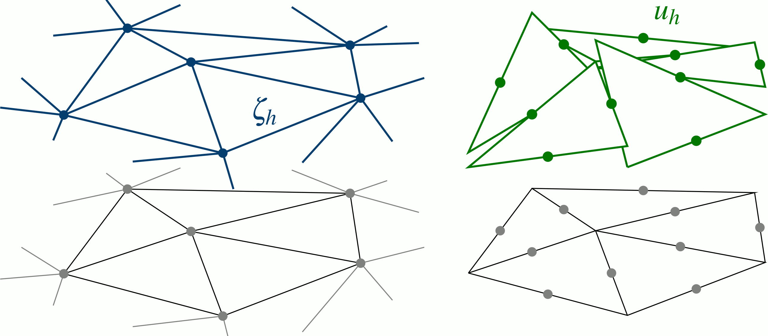
According to this approach, prior to calculating the advection term in the momentum equation, we project the velocity from $P_1^\mathrm{NC}$ to $P_1$ space in order to smooth it. This projection becomes numerically efficient by nodal quadrature (lumped mass matrix). The projected velocity is then used to estimate the advection term. Finally, the result is multiplied with a $P^\mathrm{NC}_1$ basis function and integrated over the domain . This results in a very stable behaviour.

Bottom friction¶

Manning bottom friction with a constant parameter is chosen for most calculations. Alternatively, a value varying with the surface structure can be provided.

Viscosity¶

The coefficient $K_{\!\mathrm{h}}$ for the horizontal viscosity is determined by a Smagorinsky parameterization [Sma63].

(6)¶ $K_{\!\mathrm{h}}& = c_\mathrm{smag}\,{\scriptstyle\triangle}x\, {\scriptstyle\triangle}y \,{\scriptstyle\triangle}t \sqrt{\left(u_x\right)^2 + \left(v_y\right)^2 + \frac12\left(u_y+v_x\right)^2}.$

Optionally, the standard linear viscosity $K_{\!\mathrm{h}}=c_\mathrm{lin}\,{\scriptstyle\triangle}x\,{\scriptstyle\triangle}y$ may be chosen.

Wetting and drying¶

Extrapolation from wet to dry nodes¶

For modelling wetting and drying, we use a moving boundary technique based on the “dry node concept” [LWL02]. The idea is to exclude dry nodes from the solution, but to extrapolate the elevation to the dry nodes from their wet neighbours. As this scheme is neutrally stable, it requires horizontal viscosity in places of large gradients of the solution. The Smagorinsky viscosity (6) fulfills this task while keeping the dissipation on a level that does not affect the quality of the solution.

The implementation in TsunAWI showed that in order to retain stability it has to be decided which values to extrapolate and how. Finally, linear extrapolation was chosen for the gradient $\nabla\zeta$ and the sea surface height $\zeta$ at dry elements and nodes. Furthermore, all other values at dry nodes, elements, and edges are excluded from further computations, as shown in the following figure.

../_images/wetting-drying_extrapolation.png

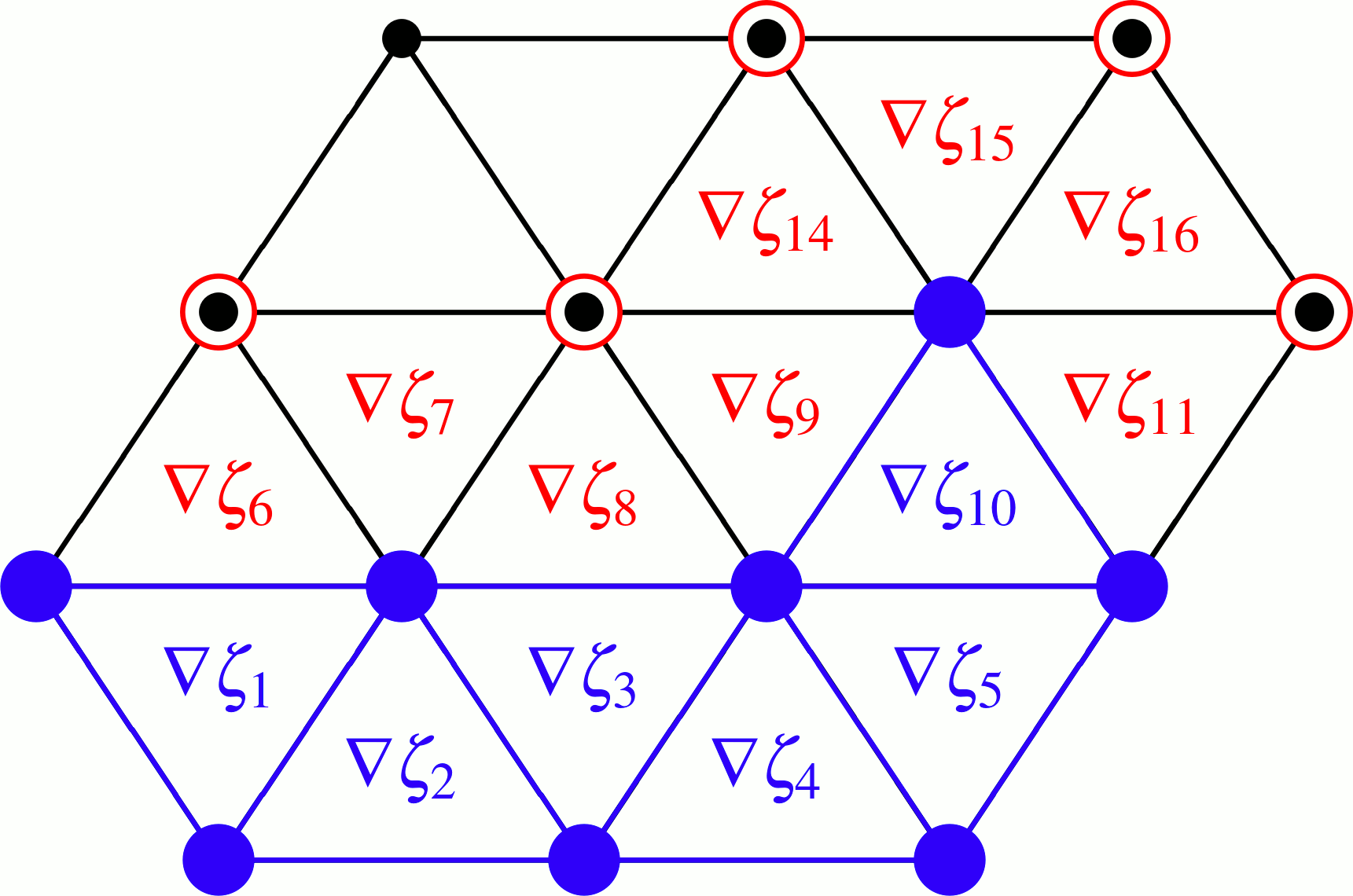
Sketch for the inundation scheme based on the extrapolation from the wet to the dry elements and nodes.

Compute $\color{blue}{\nabla\zeta}$ at wet elements, extrapolate to dry elements

${\color{red}{\nabla\zeta_j}}= \sum_{i\;\mathsf{wet}}^{i\cap j\neq\emptyset}\color{blue}{a_i\nabla\zeta_i},$

Compute velocity $\color{blue}{\vec{v}}$ at wet edges, set ${\color{red}\vec{v}}=0$ at dry edges.
Compute ${\color{blue}\zeta}$ at wet nodes, extrapolate to dry nodes

${\color{red}\zeta_n^{t+2\triangle t}}={ \sum_{m\;\mathrm{wet}}^{m\cap n\neq\emptyset}{\color{blue}a_m} \left({\color{blue}\zeta_m^t}+{\color{red}\nabla\zeta_m^{t+\triangle t}}\cdot(\mathbf{x}_n-\mathbf{x}_m)\right)}.$

GETM scheme¶

Alternatively, a linear damping factor can be employed in shallow regions [BBV04]. This scheme has many advantages regarding computational efficiency and simplicity. We have obtained promising results in test cases, however, the implementation in TsunAWI is not as fine tuned as the extrapolation scheme.

Computational mesh¶

TsunAWI works on unstructured triangular meshes that allow to cover the coastal areas with a high resolution, while the long tsunami waves in the deep ocean can be represented by a coarse mesh, thus saving computation time and memory. Here, we describe some background on what to consider when building a mesh. See Mesh files on how to specify a mesh for TsunAWI.

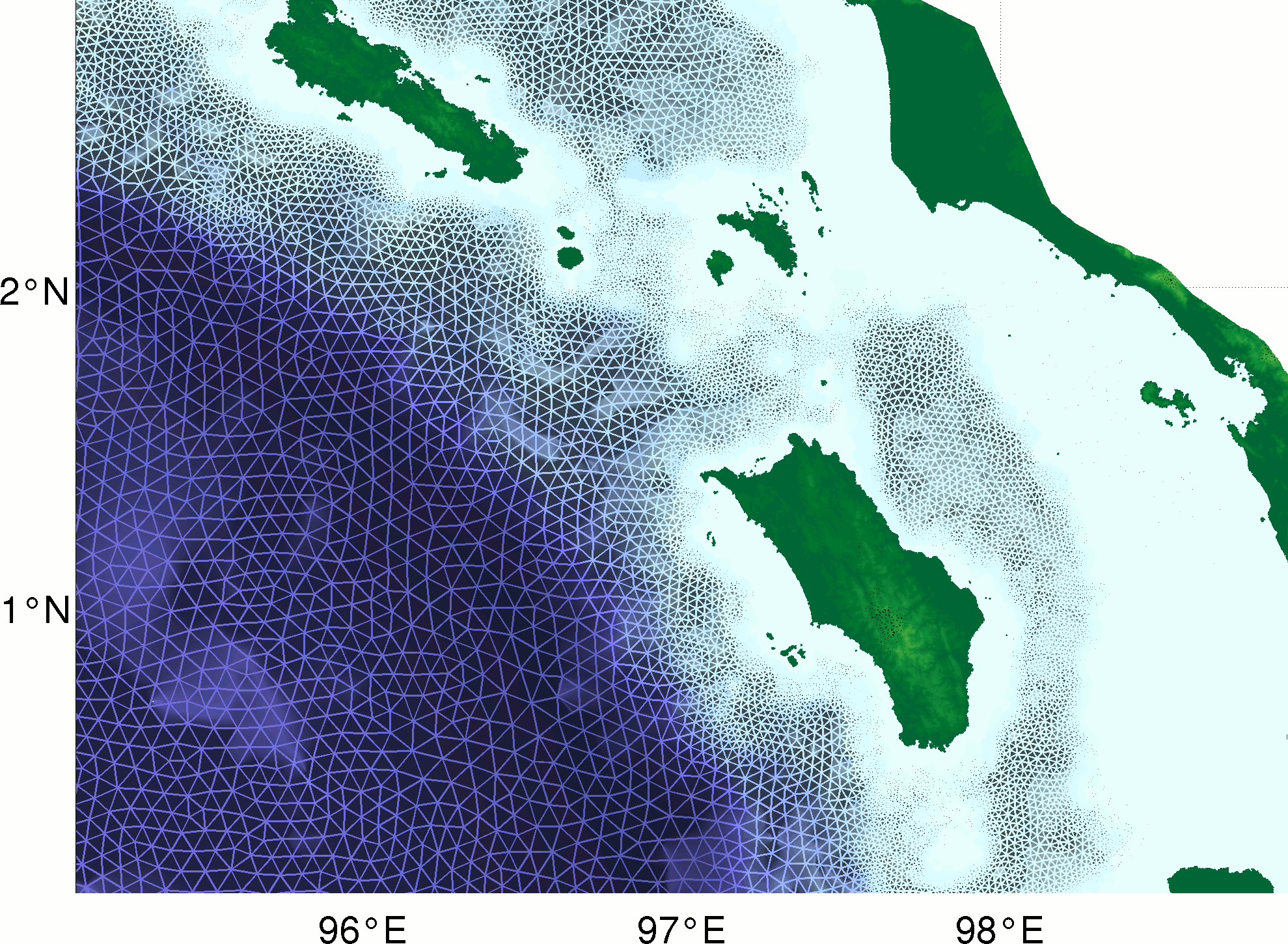
Zoom to the coast of Sumatra and the islands Simeulue and Nias in the computational mesh for the first set of scenarios for the Indonesian warning system.

Mesh generation¶

The quality of the triangulation of the model domain is crucial for the model results. The meshes used in our studies were generated with a mesh generator based on the freely available software Triangle [She96]. Starting from a model domain defined within a topography/bathymetry data set (in our case GEBCO 30”); Triangle generates a mesh based on a refinement rule depending on the water depth and prescribed by the corresponding wave phase velocity and the Courant–Friedrichs–Lewy criterion (CFL). The triangulation will be refined until the edges in all triangles fulfill the criterion

${\scriptstyle\triangle}x\leq\min\left(c_\mathrm{CFL} \sqrt{gh},\; c_g\frac{h}{\nabla h}\right)\,.$

As the Triangle output is not smooth enough for numerical experiments, several smoothing iterations are applied. Each iteration consists of edge swapping, torsion smoothing, and linear smoothing. Torsion smoothing tries to adjust the angles around each node, linear smoothing acts on the distance between nodes. These strategies are described in [FF91].

As an example, the scenarios for the Indonesian warning system have a varying resolution of 12km in the deep ocean, 150m at the coast, and 50m in project regions and around tide gauges.

Ordering the mesh for computational efficiency¶

The numbering of the nodes and elements has a strong influence on the computational efficiency. We got best results by geographically odering the nodes along a space filling Hilbert curve. Another option is to build the adjacency matrix and to employ reodering techniques like Reverse Cuthill-McKee (RCM) or Minimum Degree. In a final step, the elements should be ordered numerically by node indicees.

Performance similar to the space filling curve was obtained with Forsyth’s vertex cache optimization [For06]

Uncertainties in tsunami modeling¶

When running a tsunami simulation, please always keep in mind that many uncertainties come into play.

Initial condition:: The bottom movement due to the earthquake is usually a large source of uncertainty. In addition to a not fully known earthquake mechanism, the earthquake might trigger land slides.
Bathymetry and topography data:: The quality of the data is crucial for the result. Freely available data like GEBCO and SRTM are usually sufficient for a rough estimate of the wave height at the coast, but not well suited to assess the inundation. On a local level, the tsunami might be amplified by features like a hill, a channel, or a very steep slope that are missing in the data.
Model physics:: The non-linear shallow water equations are derived with the assumptions that the wave length is larger than the water depth and that the vertical velocity component is constant in the water column. These assumptions are no longer valid for example for water streaming through the structures of a harbour or through streets. Furthermore, additional aspects like tides are neglected.
Parameters, parameterisations, and mesh resolution:: The bottom roughness or the viscosity are physical phenomena, however, the numerical representation is a simplification and dependend on the mesh resolution.
Bugs in the code:: And, of course, it is a reasonable assumption that TsunAWI is not bugfree.

References¶

[BBV04]

H. Burchard, K. Bolding, and M. R. Villarreal. Three-dimensional modelling of estuarine turbidity maxima in a tidal estuary. Ocean Dynamics, 54(2):250–265, 2004. doi:10.1007/s10236-003-0073-4.

[For06]

Tom Forsyth. Linear-speed vertex cache optimisation. 2006. URL: http://tomforsyth1000.github.io/papers/fast_vert_cache_opt.html.

[FF91]

William H. Frey and David A. Field. Mesh relaxation: a new technique for improving triangulations. Int. J. Numer. Methods Eng., 31(6):1121––1133, 1991. doi:10.1002/nme.1620310607.

[HLRLD05]

(1, 2, 3) Emmanuel Hanert, Daniel Le Roux, Vincent Legat, and Eric Deleersnijder. An efficient Eulerian finite element method for the shallow water equations. Ocean Model., 10:115–136, 2005.

[LWL02]

Patrick Lynett, Tso-Ren Wu, and Philip Li-Fan Liu. Modeling wave runup with depth-integrated equations. Coastal Engineering, 46:89–107, 2002.

[RoedC86]

L. P. Røed and C. Cooper. Open boundary conditions in numerical ocean models. In J. J. O’Brien, editor, Advanced Physical Oceanographic Numerical Modelling, volume 186 of C, 411–436. NATO ASI, 1986.

[She96]

Jonathan Shewchuk. Triangle: engineering a 2d quality mesh generator and Delaunay triangulator. In Ming C. Lin and Dinesh Manocha, editors, Applied Computational Geometry: Towards Geometric Engineering, volume 1148 of Lecture Notes in Computer Science, pages 203––222. Springer, May 1996.

[Sma63]

Joseph Smagorinsky. General circulation experiments with the primitive equations. Mon. Wea. Rev., 91:99–164, 1963.